Mechanical Stress Computer Simulation

[joanlluch]

I thought that it would be interesting to some forum members to see what can be done on a computer in relation with mechanical stress simulation.

So I prepared some screen captures and images to show the concept and the basic steps you would follow to make a stress simulation study. I will perform this on a single part that gets solved quite fast by the hardware that I have, so I can present it in a more o less didactical way. This is not meant to be a tutorial, but just something to show the essentials. I am not an expert in any way, but someone who has taught himself out of interest. Still I will be happy to reply to any questions that I may be able to answer.

STEP 1 (The model)

You start by creating a 3D CAD model of the part that you want to study. For this example I chose a segment of pipe featuring an almost kidney shaped section. The part is made of a Stainless Steel ISO pipe, 139.7mm OD and 3mm thickness, cut in half and added a flat sheet on it through a round transition. This is the starting 3D CAD model.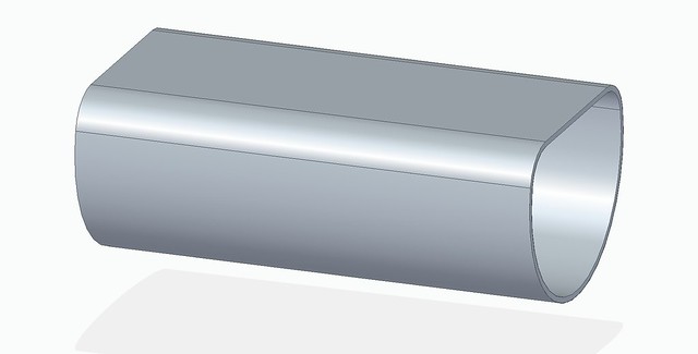

Tub by joan lluch, on Flickr

The 3D model already specifies all the geometry which the simulator will use to make the calculation. In addition you must specify a material for the part. The software will use the mechanical properties of the specified material to perform the simulation and give results.

STEP 2 (external loads)

Specify the external structural loads the parts will be subjected to. In this case, I applied a "pressure" load all round the exterior surfaces of the part. The software also allows you to apply "force", "torque", "displacement" and "bearing", so you are able to simulate a great number of real life situations. I applied a pressure of 10 bar.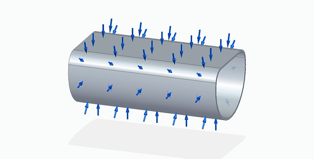

Tub-Loads by joan lluch, on Flickr

STEP 3 (constraints)

Apply constraints. This is required to instruct the software what faces on the model should be constrained to movement. The software will issue a warning and will stop computing if the part is not fully or correctly constrained. You need to apply constraints in a way that makes sense for the kind of results that you are looking for. In this example I want to study the behaviour of the part main surfaces when subjected to pressure, so I constrained the edges of the tube. The simulator will fail without these constraints because the part would conceptually be able to move in the space after applying pressure only on the external surfaces. I chose to add "fixed" constraints, other possibilities are "pined", "sliding along surface", "cylindrical", "custom". For some type of constraints you can specify further options, for example the cylindrical constraint allows you to constrain "radial growth", "rotation", and "sliding along axis" in an individual way. Again, the number of possibilities allow you to chose the right way to constrain the movement of your model in order to get the simulation you are looking for.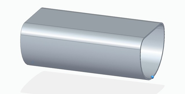

Tub-Constraints by joan lluch, on Flickr

Constraints on the picture above are represented as the blue dot that appear on the bottom right of the part. This means that this lateral surface is fully constrained, i.e it isn't allowed to move in any direction.

STEP 4 (connectors)

Next step is applying connectors. This specifes in which ways several parts are connected together. Since we are simulating just a single part for now, we can skip this step. I will come back to it latter.

STEP 5 (mesh)

At this point the simulation setup has been fully defined, and this is when the actual simulation begins. We start by computing a mesh to the model. This is performed automatically by the software but it may take some time depending on the complexity of the model being simulated. You can play with finer and coarser mesh depending on the model, your computer hardware resources, and your aim for very precise results. The smaller the mesh size the better, but you must balance it with what the computer can really do.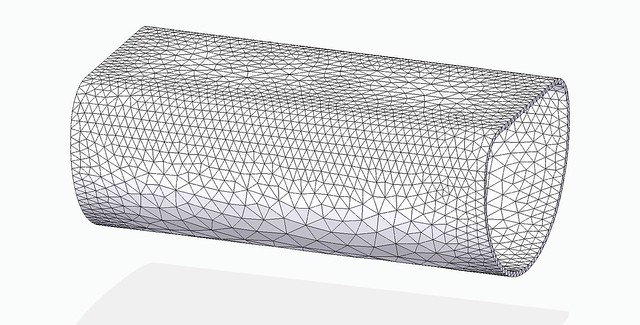

Tub-Mesh by joan lluch, on Flickr

Based on the computed mesh, and the definition of the model loads and constraints, the computer will perform Finite Element Analysis to give simulation results.

STEP 6 (simulate)

Now we are ready to run the simulation. This particular model will take just a few seconds on my computer, but time and resources go exponentially up as more parts and complexity are added to the model. The software allows you to chose several algorithms that are supposedly best suited to particular scenarios or models. Some are able to make better use of the available CPU cores in your computer. But I am not really able to tell the difference, so I always choose the default one.

SIMULATION RESULTS

Results are presented in a graphical way using colours and gradients on the model surfaces to help visualise what's going on with the parts when they are subjected to the previously specified mechanical loads. You can present results in several ways, and adjust visualisation parameters in many ways so you can really see the problematic areas and think about ways to improve them. The default display is the "Von Misses Stress" with "All Results Scale". This shows the full range of mechanical loads in the model with a multicolour scale. This mode also shows the yield stress of the material being used for simulation.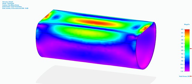

Tub-ResultsStress by joan lluch, on Flickr

A red arrow on the colour scale points to the tensile strength yield that is considered for the material that was specified. The tensile strength yield is the point where the metal starts to get non recoverable deformation. In this particular case, the simulation is telling us that there are significant areas of the part that will not be able to sustain the loads that we specified. In particular anything that is above 248MPa is beyond the load that the metal will be able to stand without permanent deformation. So results indicate that this part WILL FAIL !.

It is also possible to display a view of the deformations occurring in the part and even create a video of deformations developing as more external loads is increasingly added. Deformations can be displayed in an exaggerated way to help identify problematic areas. Next picture is a capture of deformation results. The part is slightly oriented in another way to make them more obvious: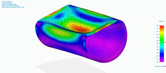

Tub-ResultsStressDef by joan lluch, on Flickr

My favourite result view, is the "Factor of Safety" view. This essentially indicates by which factor the part is safely sustaining loads. A safety factor of 1 indicates that the part is just shy of permanent deformation. A safety factor of 2 indicates that the part is subjected to half its maximum admissible yield stress, or in other words, you could increase external loads times 2 before getting the part deformed or broken.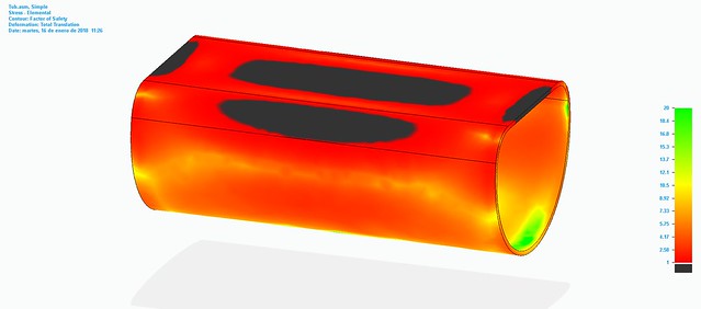

Tub-ResultsSF1 by joan lluch, on Flickr

A nice feature of all the view modes is that you can specify a different colour for overflow or underflow scale values. For the picture above I specified 'black' colour for all values below a safety factor of 1. This clearly indicate the areas where the part will FAIL, which become black coloured.


On my next post I will propose a change of the model to make it work. In particular I will be adding ribs to the tube in order to improve the model and its mechanical behaviour subjected to the same loads.

[joanlluch]

Ok, So I am now adding 'ribs' to the model that I tried on my previous post.

STEP 1 (The model)

Since the simulation software is fully integrated in the 3D CAD system, all I need to do is to draw the ribs as separate parts and add them to the assembly containing the tube in the usual way, then apply the simulation steps.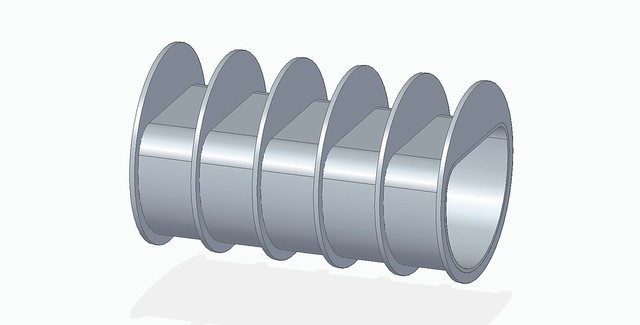

Tub-Rib by joan lluch, on Flickr

I am able to create a new simulation study based on the previous one, or just extend the previous one with added features. I usually chose to create a new one, so that the original one remains intact and I am able to possibly try different changes or additions on the model while keeping all the historical results at hand. So I start by copping and pasting the existing simulation study into a new one, and work from that for any new additions.

STEP 2 (external loads)

External loads are the same as previous model, so I do not need to add anything to that.

STEP 3 (constraints)

Constraints are also the same as the previous model, so nothing to do on this step.

STEP 4 (connectors)

Since I have added additional parts to the model, I must specify the way they are mechanically linked (or connected) among them. Connectors can be generated automatically by the software if you just want to "glue" parts with matting faces together. Since the ribs are designed to matte the surface of the tube, I can run the automatic generation of connectors. Otherwise I can create connectors manually by selecting pairs of surfaces that should become connected. There is also special connector types for "bolts" and "edge connectors". The latter is when you want to connect edges rather than surfaces.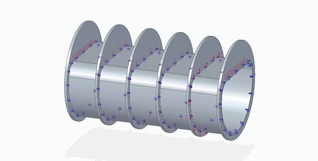

Tub-Rib-Connectors by joan lluch, on Flickr

The model with all the external loads, constraints and connectors looks like this: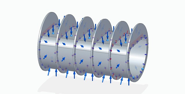

Tub-Rib-All by joan lluch, on Flickr

STEP 5 (mesh)

Now we have everything fully defined so it's time to mesh the model. This is how it looks:

Tub-Rib-Mesh by joan lluch, on Flickr

STEP 6 (simulate)

This is just running the solver and waiting for it to finish.

SIMULATION RESULTS

The "Von Misses Stress" view now show a much relaxed set of loads compared with the original model. There's no spot where loads would be higher than the tensile stress yield.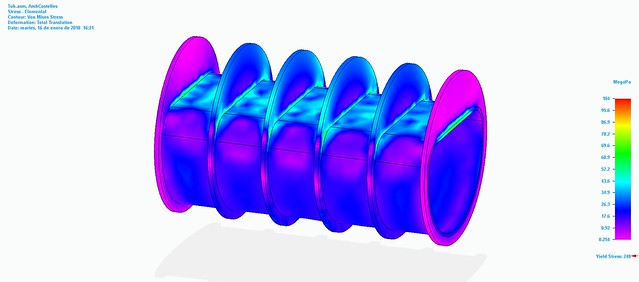

Tub-Rib-ResultsStress by joan lluch, on Flickr

The following picture shows the pattern of deformations that would occur.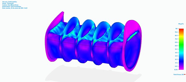

Tub-Rib-ResultsStressDef by joan lluch, on Flickr

The above is just an exaggerated view of what and where the deformations actually happen. Actual deformations are much smaller. In fact all the other views are displayed with the "actual deformations" setting. So none appreciable at all, and none permanent because as seen the material never gets stressed beyond its limit.

As said on my previous post, my favourite view is still the "Factor of Safety" with black coloured underflow values.

Tub-Rib-ResultsSF1 by joan lluch, on Flickr

The above is displayed with the scale set from 1 to 20 (safety factor). However, we may want to design our part with an intrinsic safety factor of 4, and we can check that too in a visual way just by setting the scale starting at 4.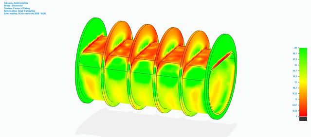

Tub-Rib-ResultsSF4 by joan lluch, on Flickr

The virtual lack of black spots indicates to us that the model is still fine with an external load 4 times the designed one. So if our design goal was for a mechanical safety factor of 4, the parts are now in accordance with our specs.

Please feel free to comment on anything that would be of interest.

Regards,

Joan

[kipford]

Nice summary. May I show a practical example of a some help I gave to someone back in November of last year. On another forum someone asked for help with checking the calculations for a boiler for a 71/4" gauge Highlander to the Martin Evans design. The original design intent was for the boiler to be manufactured from silver soldered copper, however the OP wished to use a welded steel boiler. His boiler inspector felt he was not qualified to check to the calculations and this was why he was looking for help. I offered to help as I will eventually be designing a new boiler (in copper) for an LNWR 4” Shunting Engine and this was a great opportunity to iron out the methodology. The OP had based his calculations on a number of sources:

AMBSC Code Part 2 – Steel Boilers

Recommendations by Alan Stepney

The Countryman’ Steam Manual

I am not going to discuss in detail the relative merits of any of the above, but the AMBSC code is configured to allow people without the full theoretical knowledge design a safe boiler. Note the rider here is that as far as I can tell from the data supplied the code does not take into account the weld joint design or competency of the welder which play a big factor.

What I did was to take his design and analyse it in three ways:

1. Checking his calculations using the AMBSC code

2. By hand calculation working from first principles

3. By use Finite Element Stress Analysis (FEA) of the OP that the boiler inspector can use to validate the design. As an aside I got one of our Stress Engineers at work to run the analysis separately to confirm my analysis was correct.

Anyway. The FEA methodology used was basically as Joan has shown. The basic boiler specification was as follows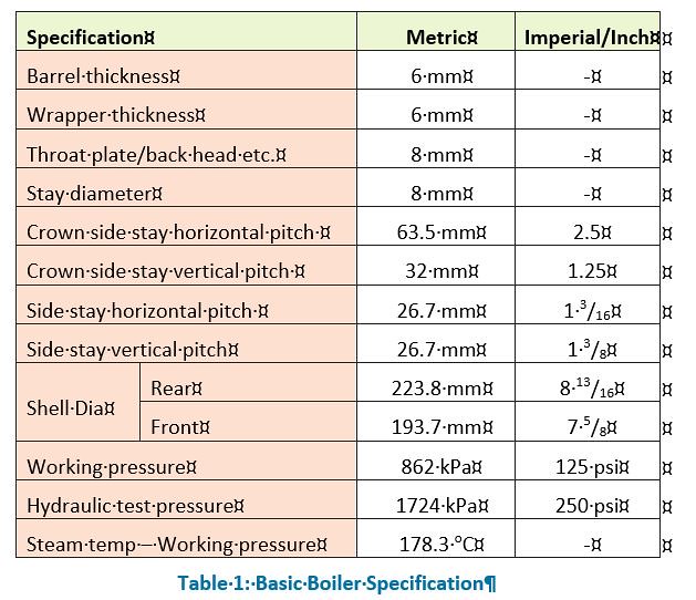


Boiler Specification by Dave Smith, on Flickr


Using the Martin Evans drawing the design was amended to suit a welded steel construction but ostensibly keeping the same stay positions etc. A sectional cross section of the 3D CAD model is shown next.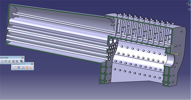


Boiler Axial Section by Dave Smith, on Flickr


The analysis method basically then followed what Joan shows in his posts above. The boiler was restrained on the smoke box end of the boiler barrel to allow the pressure to act fully over all surfaces. The next two pictures show the pressure surfaces.


Pressure Surface 1 by Dave Smith, on Flickr

Pressure Surface 1 by Dave Smith, on Flickr


The analysis results in the same as Joan shows a pretty picture with lots of colour, see below. Note I amusing max principle stress not Von Mises as you get a more pessimistic (higher stress) result. You have to now interrogate the model to find out what is going on. Each part is reviewed for it maximum stress. I will not go into it now but the validity of the result is also reviewed to establish if the actual peak stress is realistic or a function of the accuracy of the model and the analysis has been carried out. Simply put if you are not careful it is shit in = gospel out. I have seen this happen too many times over the years.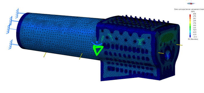


Stress 1 by Dave Smith, on Flickr

The boiler was stressed at both the working and hydraulic test pressures. But the analysis does not take in account the effects of material properties reduction at temperature, manufacturing methods or corrosion (as it is a steel boiler). The two tables below show the analysis results corrected for the knockdown factors and the resulting reserve factor (RF) for each part. In this case I used the 0.2% proof stress for both the working and hydraulic pressures. You could use the ultimate tensile stress for the hydraulic analysis, but that potentially allows plastic deformation which I did not want to see. I consider the hydraulic test to be a proof test. Because of the level of knockdowns used and the use of the 0.2% proof stress it is acceptable for the RF not to be <1.5. If you look at the results you find the only dodgy parts were (some not all) of the stays. This was simply remedied by increasing the stay diameter by 1.5 mm, the effect on the stay stress being a simple hand calculation and not requiring a repeat analysis.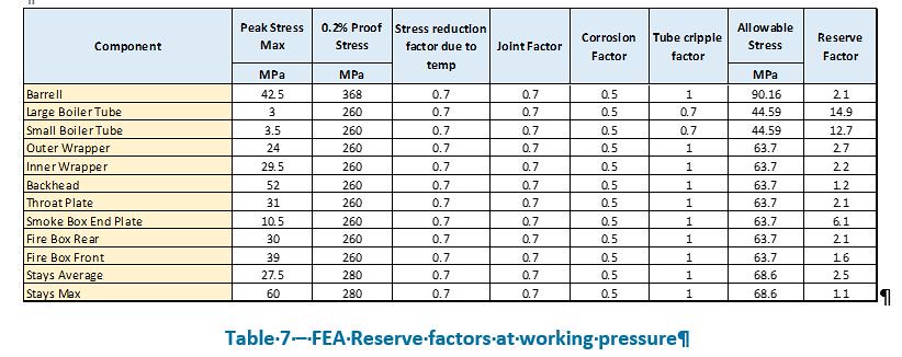


Results Working by Dave Smith, on Flickr

Results Hydraulic by Dave Smith, on Flickr

Hope this of interest.

Dave

[joanlluch]

Hi Dave,

Thanks for sharing this.

I will also have a welded boiler. Unfortunately I can't simulate it as a whole because I found that the software would need a lot more memory to complete the entire analysis and my current hardware does not allow more than 8Gb. So I am simulating it by its individual components instead. I essentially constrain individual components, or sets of them, in ways that would not affect the global results and I study the individual components individually.

I have a question about your simulation. For the stress analysis I let the software pick the default yield strength of the material being used, so it is identical for all the components because they are all the same material. My question is, what's the reason for you to use a different value for the 0.2% proof stress depending on the component?.

Please correct me if I am wrong. I think that the stress results are always proportional to the external loads, so in fact I believe there's no need to run a different simulation for the working pressure and the hydraulic pressure, as both results are simply proportional. I am a fan of the 'safety factor' view because it presents data in a rather independent way. Ultimately, it's just a matter of deciding what safety factor I would accept as a minimum value depending on the external loads that I have applied, and the reduction factors that I may consider on each case. I suppose doing it this way is not the most elegant or academic, but I think it gives the same information.

Joan

[kipford]

Joan

Thanks for the comments.

I do not know what software you are using but the analysis was carried out on a LenovoW530 with 8Gb of ram, it runs it quite happily. The analysis file size is around 100Mb. I have a new computer at home and will try running on that to see what happens.

The reason for different proof stress values, is that the builder had already had the boiler barrel rolled and welded and hence the allowable stress reflects the grade of material used. For the rest of the boiler I wanted to allow the a choice of materials to be used, hence went for mild steel. If the builder/welder wants to use higher strength materials then the analysis remains valid, nothing complicated.

You are correct you only need to run it once, then you can factor the results for the different pressures and that is what I would have done in my normal work environment. However here I had to produce a report to show a boiler inspector with limited (by his own admission) technical knowledge that the boiler was theoretically structurally sound. It was easier to do a second run, than have to try and explain that this is a linear analysis and hence it is acceptable to factor the results. It only takes about 20 minutes to run the model so it was not a problem. For the same reason noted above the knock down values were clearly presented to show their effects.


Regards

Dave

[joanlluch]

Hi Dave,

I use Solid Edge ST10 as software, and an Apple iMac 21.5" from 2014 running Microsoft Windows 7, with Intel Core i5 (four cores) at 2.7GHz, 8Gb RAM, and SSD drive. Memory can't be upgraded because the computer was one of the cheaper offers of the time.

My boiler is not conventional, as it is based on water tubes. I think this adds more complexity to simulation. Also the boiler wall thickness is only 3 mm, as it's made of Stainless Steel. The picture below is one of the more complete simulations that I was able to perform:

Simulacio-InteriorTubSF3 by joan lluch, on Flickr


My problem is that I have to select a too small mesh size to prevent the software complaining due to the small thickness of the parts. The simulation above only covered the inner boiler walls. It took 20 minutes, but the software used up to 30GB of virtual memory. The disk activity due to virtual memory page faults was tremendous. I can't really do more than that unless I am able to increase the mesh size or use a computer with more memory.

Joan

[runner42]

Hi Joan,

an interesting subject. FEA using computer software is used extensively in the Defence Industry and during my tenure working for Maritime Systems Division Submarine Branch I had the responsibility for reviewing a number of FEAs performed on the platforms integrated into the submarine. These platforms were resiliently mounted so that a shock from say a mine sustained by the hull was not transmitted to equipment mounted on the platform or conversely vibration from rotating equipment on the platform was not directed to the hull which would radiate the noise and add to the noise signature of the submarine. These platforms were large so physical shock and vibration testing could not be performed on these so FEAs were undertaken. I am no expert, but was able to review these against certain criteria and if I had any concerns I would ask the cognizant engineer to clarify the results. The accuracy of the FEA is predicated on the ability of the software assuming that all the correct parameters were inputted as required.

Also understanding the software and how it operates is a pre-requisite, that was not my responsibility that being the engineer performing the FEA.

Your example covers stress analysis of kidney shaped tube and with fins added and the results of the FEA indicate I assume that the structure is able to withstand the stresses that you have subjected it to. Can you extend the calculations further to determine what the failure load would be and determine the failure mode of the structure? 

FEAs are useful in other applications such as heat transfer and fluid flow, could you produce an example of within a locomotive boiler the heat transfer and identify and potential hotspots?

Brian

[joanlluch]

Hi Brian,

Thanks for your input. I'm not really an expert, but I can try to explain what I understand of it.

My examples attempt to show failure of the original kidney shaped tube and success of the same structure after adding the ribs. The simulation results show whether the structure would withstand the external stresses and where the failure would first occur, but some interpretation is required. There are several ways to look at it but I think most people look at the "stress" results. You need to consider that for calculation purposes the software considers an unlimited yield stress for the material, i.e it assumes it will not break, and it shows the resulting stress values in a coloured scale. This allows you to identify where the actual stresses would go above acceptable.

On the first scenario (initial post) the max stress is represented in red colour on the "von misses stress" picture. The max value is 451 MPa. On the other hand, the material is supposed to withstand 248MPa without permanent deformation (strength yield). This is indicated with a red arrow next to the colour scale. Anything above that value, that is: most of green, yellow, orange, and red coloured areas, are above what the material can get. These are failure areas.

Since the computational model is lineal, you can just recalculate the max external load that the structure would withstand by a simple rule of three. On the first scenario the applied external pressure was 10 bar. The structure gets to a max of 451 MPa. The max allowable yield stress for the material is 248 MPa. Therefore, this structure can withstand 10 x (248/451) = 5,5 bar. This is of course without applying any safety or reduction coefficient at all, but you get the idea. The more stressed areas would still be in the same places as indicated by the colour code. At 5.5 bar all stresses would be accordingly reduced by a factor of 248/451 = 0.55 . There's really no need to repeat any simulation for a particular structure because results are all lineal, and you can always apply factors to get your desired conclusions.

Back in my university days I had a course on computerised heat transfer simulation which I got the very top mark. This was in the late 80's. To be honest, I got such an outstanding mark because anything involving software development was easy to me, not because the subject of heat transfer was particularly interesting to me. Actually, I refused an offer to enter the heat transfer department as an investigator and teacher, because I was more interested in computer language compilers design. After so many years, I only recall the very basics of what was taught in the heat transfer classes as I did not really need that during my professional career. Of course, many things have changed since then, and it is no longer necessary to have computer programming skills to produce a heat transfer simulation, if you own the proper software. But I have not looked at it again and I am not currently able to produce such an example, which incidentally would be a very interesting exercise if someone else is able to work on it.

Joan

[joanlluch]

Just in case someone would like to see an arbitrary example of heat transfer and fluid flow analysis, I found a couple of videos on youtube to make it more convenient for all.

youtu.be/Mu2R0xFJtBA

youtu.be/E5JYSV5Jj1c

Joan

[runner42]

Hi Joan,

thanks for the response, from your university days you have demonstrated that you have a good academic grasp of heat transfer and fluid flow, combined with your interest in computer software for producing FEAs. The example that I alluded to in the locomotive boiler construction has a real life application to the making model locomotive copper boilers that comply with the AMBSC Code Part 1. This code requires at para 3.12 that tubeplates shall have a minimum ligament of 4mm. The ligament is the separation distance between tubes and flues and the rationale for establishing this criterion is that particularly at the firebox tubeplate water flow between the tubes and flues could be affected such that a hot spot is generated due to the absence of cooling water and cause premature failure of the silver solder joint. 

Now this 4mm ligament may have been arbitrarily established by the committee as being the minimum distance that would occur in a 5" gauge boiler and not based on real engineering analysis. This assumption may solicit an adverse response from those who have intimate knowledge of the background reasoning for establishing a minimum 4mm ligament. However, many model locomotive boilers particularly in 3 1/2 gauge and smaller will by necessity have a ligament under 4mm. Rob Roy by Martin Evans is such an example.

If an FEA is performed on a representative boiler design it may be demonstrated that a smaller ligament is permissible. 

Brian   

[kipford]

Brian. The AMBSC code will almost certainly have been written to allow people with limited technical experience in stress analysis to design a safe boiler. This is suggested in the work I did to stress a steel boiler. One example is the minimum diameter for boiler stays being 19mm! It is just about workable in 71/4 gauge but produces significant blockage. In the smaller gauges I would think this would become a show stopper. By carrying out a full analysis it can be shown that even with considerable reduction factors for temperature, corrosion etc applied the stay diameter can be significantly reduced from that in the code. Hence I would expect the ligature distance to be able to be reduced if a proper analysis is conducted. After all the stress in a 3mm thick tube plate will Increase by the cube of the thickness ratio for a tube plate of 6mm thickness with the same ligature width. If you want I could have preliminary look at the stress involved if you want.
Regards
Dave

[joanlluch]

Hi Brian,

I think that a too small ligament can definitely have a negative influence on the boiler for the reasons that you mention. If tubes are too near from each other, water flow can be very reduced around the firebox tubeplate. Also increased temperature in that area can promote scale deposits which will in turn isolate the inner walls of the boiler, thus getting the tubeplate even hotter. But that's just pure speculation based on what I think that could happen, this is not saying that a smaller ligament wouldn’t be ok, it probably is, because as shown by Dave normalised boilers are already very over-dimmensioned and safe.

I am pretty sure that proper and complete boiler simulation including not only stress computation but also mass flow and heat transfer simulation would debunk some of the currently accepted principles. If some day such a study is thoroughly performed by somebody, it might get active opposition and require some time to be accepted, but it can set a change in boiler design and inspection criteria.

Joan

[joanlluch]

Just as a matter of information about some additional possibilities regarding the subject of this thread.

In cases where the model is fully symmetrical with respect a particular plane, a simulation of just half the model can be performed. This can dramatically enhance simulation performance because you end having half the number of elements and nodes. Solving time increases exponentially with the number of nodes, so it's not a matter of just getting results with half the processing time or computer resources, but much better than that. (Thanks to Eric 'thumpersdad' for his useful contributions on my build thread, who helped me to figure out the right way of doing it)

Eventually, the example simulation that started this thread is a perfect candidate to show this. Both the model and the applied loads are perfectly symmetrical with respect to the XZ plane. Thus we can take advantage of that to perform a stress study on just half of the part, while still getting all the information.

Changes to the model are as follows:

1 - The model has been cut in half along the symmetry plane, in this case the XZ plane. This is the resulting mesh.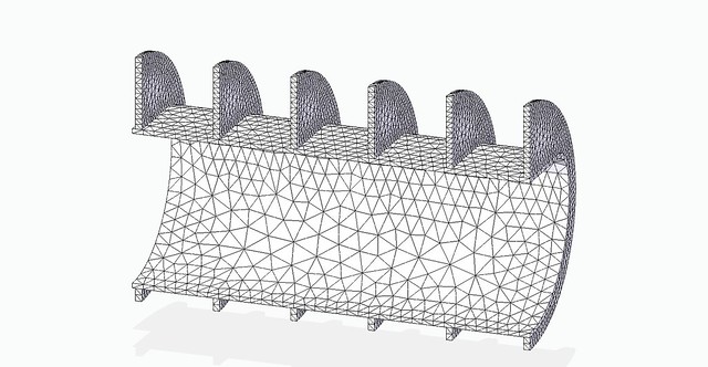

TubPartit-Mesh by joan lluch, on Flickr


2 - Loads are identical but of course only applied to the half model.

3 - Constrains are the same, but again only operating on the half model that is left.

4 - New "sliding along surface" constraints have been added to the cut surfaces on the symmetry plane. We need to do so to prevent deflection across the symmetry plane while allowing deflection in the plane, and this is the key for enabling symmetrical part studies.

TubPartit-SConstraints by joan lluch, on Flickr


These are the results:

The following picture shows the pattern of deformations that would occur. As expected deformations are the same than the ones occurring on the previous model. Also as expected, max stress resulted in a very close value, 108 MPa compared to 104 MPa and it happened in the same exact point. The value difference is attributable to the automatic mesh size that was used on both models, which eventually resulted in slightly smaller elements around the more stressed point for the half model.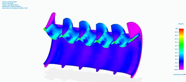

TubPartit-ResultsStressDef by joan lluch, on Flickr


Finally, the next picture is my favourite "Factor of Safety" results. Again, virtually identical to the full model one.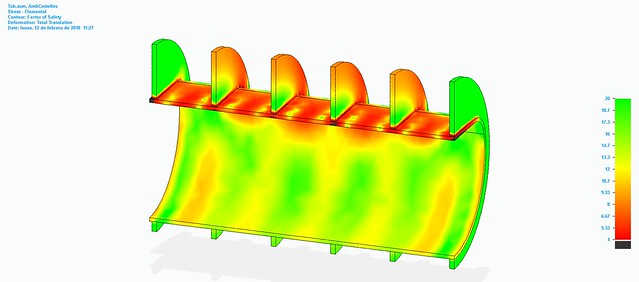

TubPartit-ResultsSF4 by joan lluch, on Flickr

Joan